Next: Harvesting
Return to: Limits on Growth
Up: Outline

Equilibria, Stability, and Phase Space

We now know that we can find equilibria solutions to a differential equation by finding values of the population for which dP/dt=0. But we also observed that the two equilibria solutions for the logistic population model differ: for one equilibria, nearby trajectories (solutions to the differential equation) are "attracted" to the equilibrium; for the other equilibrium, nearby trajectories are "repelled." We call the first case a stable equilibrium (also called a sink) and we call the second case an unstable equilibrium (also called a source).

In the real world, we will almost never observe an unstable equilibrium solution. For example, if a ball is pushed down a hill as in Figure 1, it may end up in the positions indicated by Q or S, but it would be a lucky push indeed that results in the ball being positioned exactly at R. For this problem, the positions Q and S are stable equilibria for the ball, whereas R is an unstable equilibrium. Even if we carefully place the ball at point R, a gentle breeze or earth tremor will cause the ball to move away from R. In contrast, placing a ball at point Q or S will result in the ball staying near that stable equilibrium, even on a gusty day.

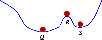
Figure 1: Equilibrium positions for a ball on uneven terrain.

Notice that geometrically, it is easy to tell the difference between the stable and unstable equilibrium positions of the ball in Figure 1. At the stable positions, the terrain is concave up, whereas at the unstable equilibrium, the terrain is concave down. The next question asks you to generalize this observation to the logistic model

dP/dt = k P - A P².

Note that the right-hand side of the logistic equation is solely a function of the current population P, so let's define F(P) = k P - A P². As before, let's call the two solutions to F = 0 C and E, with C < E (See Figure 2). We suspect from numerical experiments that C is an unstable equilibrium. By definition, this means that if we choose an initial population to be C + a where a > 0 is a small number (in particular, a < E), then we expect dP/dt evaluated at C + a to be positive. Therefore the population will increase, thus driving it away from C. This argument can be made rigorous by substituting the value of C into F(C+a) and showing that the resulting number is positive for all small values of a > 0.

We say that F defines a vector field on the phase line. At each point where F > 0, we picture a small vector pointing to the right (the positive P direction) based at that point, and we let the length of the vector correspond to the magnitude of F at that point. Similarly, at each point where F < 0, we picture a vector pointing to the left. At equilibria, we imagine the zero vector, since the magnitude of F at equilibria is zero.

These vectors give us geometric intuition into the questions: if a population is P, will the population increase or decrease? Will it change quickly or slowly?

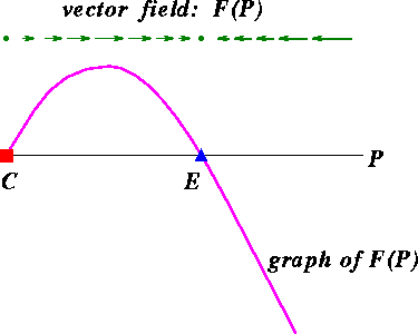
Figure 2: The vector field F(P) on the phase space gives a geometric interpretation of how solutions to a differential equation evolve.

Question 6

Construct an argument to verify that the equilibrium E is a stable equilibrium. Note this time that a may be either positive or negative.
Geometrically describe and sketch what a vector field looks like in the neighborhood of a sink. In the neighborhood of a source?
How can you determine the stability of an equilibrium by looking at the derivative (with respect to P) of the vector field? Relate this result to the physical interpretation of stability for a ball on a hill (See Figure 1) based on the concavity of the terrain. (Careful! Making the connection to a "second derivative of something" is trickier than it looks. A hint is to think of the vector field as giving a force, but Figure 1 shows the graph of a so-called "potential". Start by sketching the "force field" (also known as the vector field) for Figure 1.)
You are modeling two different populations. The net birth rate and coefficient of overcrowding for the second population is exactly twice that of the first population. Compare the location of equilibria and sketch the vector fields for these model populations. By looking at the vector fields can you determine which population is which? Can you determine which population has the shorter expansion phase?

Question 7

We've been considering solutions to differential equations that are functions of time. That means that we can also consider the solution to be the parametrized path of a particle as it moves along the phase line (the P-axis). Use the Population Simulator to generate trajectories of the logistic model and simultaneously display the solutions on the phase line.

As you generate trajectories, vary the length of time over which you follow the solution. Also vary the initial population, the growth rate, and the coefficient of overcrowding. To help you track the parametrized path corresponding to the last trajectory you generated, only the last initial condition is used to plot the path of the particle on the phase line. This path shows up in red.

Based on your observations, what is the relationship between the graph of the function P(t) and the parameterized curve on the phase line that describes the same solution?
A friend of yours who is not taking calculus looks over your shoulder as you are doing this lab and asks you, "How long will it take a population that does not start at equilibrium to reach equilibrium." Craft a response to this question that is accessible to someone who has not had calculus.

Next: Harvesting
Return to: Limits on Growth
Up: Outline

The Geometry Center Calculus Development Team

The Geometry Center Home Page