Geisow's Algorithm (Geisow)

Overview

This algorithm (also known as the "2D Bernstein Method") traces the level set of a POLYNOMIAL function of two variables. That is, given a polynomial from R^2->R, this function computes the algebraic variety associated to that polynomial. This algorithm should NOT be used on functions that are not polynomials!

How Geisow's Algorithm Works

Geisow's algorithm traces the zero set of an arbitrary polynomial curve in a specified region of x,y space. It represents the polynomial in the Bernstein basis
{ choose(N,i)(1-x)^{N-i}x^i },
because the coefficients of the polynomial in that basis have the property that if ALL Bernstein coefficients have the same sign (pos or neg), then the polynomial does not have any zeros on the interval [0,1]. (The converse does not hold: there are Bernstein polynomials with coefficients of different signs that have no zeros on [0,1].) The algorithm is therefore:
     Compute coefficients of polynomial in Bernstein form.
     Check coeffs of 2D Bernstein polynomial  
     if they all have the same sign,
        poly has no zeros ==> DONE
     else
     {
        look at first partial derivatives (as Bernstein polys)
        if they have coeffs of same sign
           poly is monotone, therefore find zero and draw soln.
        else
        {
            if we are in a small region of space, 
                draw linear approx to poly
            else
                chop 2D region into 4 subregions
                recursively generate curve for those regions
        }
    }
End result: We either
  1. draw linear approximation to level curve
  2. give up because we've reached resolution limit
  3. throw the rectangle out because there is no root in the rectangle

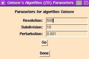
Geisow Panel

The panel that controls Geisow's algorithm.


Controlling the Algorithm From Pisces

The Pisces panel to Geisow's algorithm has 3 parameters:
Resolution
This parameter determines the size of a "small" region of space. Specifically, let L = minimum side length of initial bounding box. We will subdivide the initial bounding box into subregions until we have a subregion with side length less than L /Resolution. We will then no longer divide that region.
EXAMPLE: If you begin with a bounding box of unit length and if Resolution = 100, then we will stop subdividing space when we have a region with side length > 1/100.
DEFAULT VALUE: 500
Subdivision
This parameter is similar to the one above, except that if we let L as above, then if we have a region of space with side length less than L / Subdivision, then we assume that we can approximate the solution curve linearly on this domain. If Subdivision is equal to Resolution, then we will not fill in any of the solution until we have subdivided as far as possible. Usually, however, we want to put in pieces of the solution curve (when applicable) before subdividing to the limit, so we typically set Subdivision to be less than Resolution.
DEFAULT VALUE: 10
Perturbation
Sometimes symmetries in the polynomial being studied give us a misleading view of how the algorithm behaves. For example, if the polynomial is singular at the origin, then the algorithm will "locate" the singularity by virtue of the fact that the singularity was on one of the grid points for the algorithm. In order to restore genericity, we perturb the initial grid randomly. The size of this perturbation will be smaller than the value of Perturbation.
EXAMPLE: A user has the bounding box set for [0,1]x[0,1] with Perturbation=0.1. Then the algorithm will compute a new bounding box with xmin chosen randomly in the interval [-0.1, 0.1], with xmax chosen randomly in the interval [ 0.9, 1.1], and similarly for ymin and ymax.

Known Bugs

Coefficients for the polynomial are determined numerically, so any coefficient that has a magnitude less than about 1.0e-8 will get truncated to 0.

The routine does not verify that the current function is a polynomial. This is because a function like x + y^2 + A*sin(x) may or may not be a polynomial, depending on whether A=0, and whether x is a variable or a parameter.

Please send bug reports to software@geom.umn.edu.

Acknowledgements

The algorithm was implemented by Frederick J. Wicklin.

The code is based on an algorithm developed by A. Geisow in his 1982 PhD thesis, "Surface Interrogation," University of East Anglia, (UK)

Dr. Ralph Martin (Dept of Computing Maths, University of Wales College of Cardiff, Senghennydd Rd, Cardiff, CF2 4AG, United Kingdom) kindly gave the Geometry Center code that implemented this algorithm. The code was originally written for Sun PHIGS. Many thanks to Drs. Geisow and Martin for agreeing to allow their code to be incorporated into the Geometry Center code.


Next: A Predictor-Corrector Algorithm
Previous: User Interface
[Pisces] The Pisces Home Page
Comments to: pisces@geom.umn.edu
Last modified: Tue Nov 28 10:06:19 1995
Copyright © 1995 by The Geometry Center, all rights reserved.