Two-Parameter Continuation Algorithm for Surfaces
Overview
This algorithm traces the level set of a smooth
function f: R^{n+2} -> R^n. For n=1, a typical example is
the 3-D sphere defined by x^2 + y^2 = z^2 = 1.
For n=2, an example is the flat torus in 4-D defined by the common zeros of
x^2 + y^2 = 1 and z^2 + w^2 = 1.
How the algorithm works
The basic idea is due to Mike Henderson at IBM Watson Research Center:
- Find a point p on the surface;
- Determine the tangent plane to the surface at p;
- Create a disk on the tangent plane at p;
- Project a point from the perimeter of the first disk
down to the surface (call the point q);
- Determine the tangent plane at q;
- Create a second disk on the tangent plane at q;
- Intersect the second and first disks;
- Store the intersection points;
- Choose an intersection point, u;
- Determine the tangent plane at u;
- Create a new disk centered at u;
- Intersect the new disk with the previous disks;
- Go to step 8
Although a disk is defined on a tangent plane, the implicit function
theorem tells us that the surface is locally a graph over the tangent plane, so we may visualize the surface by thinking of each disk as projecting onto the surface to
create a local coordinate patch on the surface.
Step 1, finding a point on the surface, is typically accomplished by using Newton's
method to iterate a point in the domain onto the surface.
The steps in which the algorithm determines a tangent plane are
accomplished by determining an orthonormal basis for the kernel of
Df. These vectors are tangent to the surface since they are
orthogonal to Df (which, for n=1, is just the gradient).
Step 3, creating a disk, is accomplished by using the tangent vectors
axes of an ellipse. Two ellipses are intersected by solving a quartic
system determined by the equations of two ellipses. So that we have a
consistent coordinate system, one of the disks is projected onto the
tangent plane of the other.
The version of this algorithm that is implemented in Pisces attempts
to intelligently implement this basic strategy by
- Finding special points from which to begin tracing the surface.
(Note: Finding special points is work in progress.)
These special points include
- turning points
- boundary points
- singular points
- Detecting isolated singular points and singular curves
on the surface.

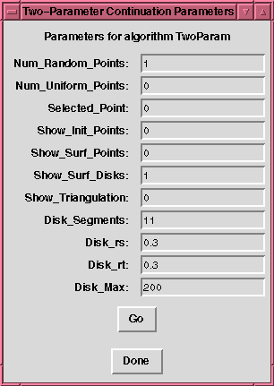
The panel that controls the two-parameter continuation algorithm.
Controlling the Algorithm from Pisces
The Pisces panel for the two-parameter continuation algorithm has
the following parameters which may be set by the user:
- Num_Random_Points (default value: 1)
-
The number of random points in the domain to use as seeds for Newton's method
in an attempt to iterate onto the surface.
If the iteration onto the surface is successful, the surface point is used
as an initial point for a tangent plane and disk center. Currently, the
algorithm only requires one initial point for connected surfaces. If the
projection fails (ie. a bad random point is selected), no action takes place
and the user needs to press the Go button to execute the algorithm again.
- Num_Uniform_Points (default value: 0)
-
The number of uniform grid subdivisions in each domain variable. For example,
in a domain R^3, selecting 2 subdivisions produces 2x2x2 = 8 points.
Currently, the grid subdivision is implemented for R^3 and needs to be developed
for R^n.
- Selected_Point (default value: 0)
-
Set this flag to 1 to force the algorithm to obtain the initial point from
the Model.Domain_Value array which can be set by the user via the Pisces Tcl shell,
or by clicking in a 2D graphics window with the left mouse button.
- Show_Init_Points (default value: 0)
-
Set this flag to 1 to display all points on the surface that were used
as starting points for the algorithm.
- Show_Surf_Points (default value: 0)
-
Set this flag to 1 to display all initial points on the surface.
- Show_Surf_Disks (default value: 1)
-
Set this flag to 1 to display all disk patches (edges only) on the surface.
- Show_Triangulation (default value: 0)
-
Set this flag to 1 to compute and display a triangulation of the surface.
Currently, the triangulation is updated every time a new disk is added to
the surface.
- Disk_Segments (default value: 11)
-
The number of line segments used for a polygonal approximation of a disk.
- Disk_rs (default value: 0.3)
-
Magnitude of the major axis for each elliptical disk.
- Disk_rt (default value: 0.3)
-
Magnitude of the minor axis for a disk.
- Disk_Max (default value: 200)
-
Maximum number of disks to compute.
Known Bugs
The first version of the surface triangulation
algorithm has missing triangles or holes under specific geometries,
most notably, when closing a surface such as a sphere or torus in 3D.
Please send bug reports to
software@geom.umn.edu.
Future Work
Improving the triangulation. Improving the speed of the algorithm,
especially when intersecting one disk with all existing disks.
Acknowledgements
This algorithm was implemented by Nicolas
Vera and Rick Wicklin. Much was learned from an earlier
implementation due to Wicklin and Dan Krech. The continuation
algorithm is based on a paper by Mike Henderson - "Computing
Implicitly Defined Surfaces: Two Parameter Continuation", IBM Research
Division, March 1993.
For questions about this implementation, contact
Frederick J. Wicklin.
Next: The Model Panel
Previous: User Interface
![[Pisces]](../../../pix/pi.gif) The Pisces Home Page
The Pisces Home Page
Comments to: pisces@geom.umn.edu
Last modified: Tue Jun 4 16:34:59 1996
Copyright © 1995 by
The Geometry Center,
all rights reserved.

![[Pisces]](../../../pix/pi.gif) The Pisces Home Page
The Pisces Home Page