The Pitchfork Bifurcation
In this section we compute a bifurcation diagram for a family of
one-dimensional differential equations. In particular, we
compute the location of equilibria for a one-parameter family, and compute the
saddle-node bifurcations for this family.
Start a new session of Pisces, and open the
Model Panel, the
Predictor-Corrector
Control Panel,
and the
View Window.
Setting up the Model
Select the DS Pitchfork model from the
Model menu on the Main Panel.
We will study the three-parameter family of vector fields on the line
given by
x^3 - mu x + alpha + beta mu
as the parameters mu, alpha and beta
are varied.
Computing a Locus of Equilibria
We wil compute the locus of equilibria for this vector
field in (x,mu)-space. To begin, we must tell Pisces to compute equilibria
and also to inflate the
domain by the parameter mu.
- Create a Derived Model
- Select Derived Model from the
Settings menu on the Main Panel. The
Derived Models Panel
will appear. On this panel, select the menu item labeled
Fixed Points ODE, then press the Update
button that appears.
- Inflate the Model Domain
- At the bottom of the
Model Panel, press the Permute button to bring up
the
Permutation Panel. Use the Permutation Panel to add
the variable mu
to the domain. Press the OK button in order to
apply the permutation.
- Compute the Zero Set of the Derived Model
- Change the following parameters on the
Predictor-Corrector Control Panel:
- Uniform_Points = 0
- Boundary_Points = 3
- Turning_Points = 3
- Singular_Points = 1
Now press Predictor-Corrector's
Go button.
Change the Hor and Ver
coordinates of the View Window in order to
project the solution curve onto
(mu,x)-space. This curve should look like
the pitchfork below (though colors may be different).
For mu<0, the vector field has only one (unstable) equilibria;
for mu>0, there are three equilibria (two unstable; one stable).
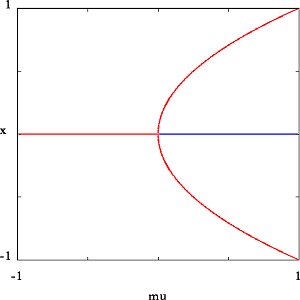
A Locus of Equilibria.
One-Parameter Animation of a Bifurcation Diagram
If the parameter beta is nonzero, the x -> (-x)
symmetry in this problem is broken. This symmetry-breaking bifurcation is
discussed in Chapter 1 of
M. Golubitsky and D. Schaeffer,
Singularities and Groups in Bifurcation Theory, I,
Springer, 1985.
To view the symmetry-breaking bifurcation, first make sure that the
Predictor-Corrector parameters are set as indicated above. Open the
Animation Panel
by selecting Animate from the
Utilities menu of the Main
Panel. Animate the parameter Model.beta in eleven (11)
steps within the interval [-0.3, 0.3], using the
Predcorr algorithm.
What you will see is a pair of nonsingular curves transform into a
singular (symmetric) curve and then back into nonsingular curves.
Computing Saddle-Node Bifurcations
We will compute a curve in
(x,mu, beta)-space corresponding to saddle-node
bifurcations. Geometrically, these are points on the curves
of equilibria for which the curve is turning with respect to the parameter
mu.
As in the previous problem:
- Create a Derived Model
- On the Derived Models Panel,
select the menu item labeled
Saddle Node ODE, then press the Update
button that appears.
- Inflate the Model Domain
- At the bottom of the
Model Panel, press the Permute button and
use the Permutation Panel to add
the variable beta
to the domain. Press the OK button
to apply the permutation.
- Compute the Zero Set of the Derived Model
- Press the Go button in the
Predictor Corrector
Control Panel. Change the Hor and Ver
coordinates of the View Window in order to
project the saddle-node curve onto
(mu,beta)-space.
The saddle-node curve separates the parameter space into four regions.
A saddle-node bifurcation occurs for parameter values on the
curve.
If Geomview is installed on your system,
you can view the saddle-node curve in (x,mu,beta)-space.
Launch Geomview by selecting
the Geomview item from the Output menu.
When Geomview appears, it should show a three-dimensional image of
the saddle-node curve. If it does not, press the
Close button on the Main Panel and then
reopen the connection via Output->Geomview
in order to force Pisces to resend its current graphics buffer.
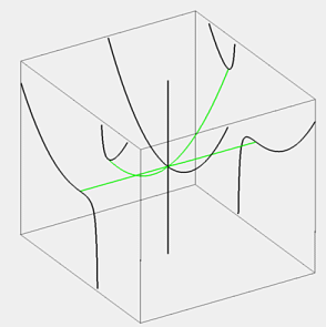
A Saddle Node curve in (x,beta,mu)-space. Three
curves of equilibria for fixed beta are included to show
that the saddle-node curve corresponds to turning points of the
curve of equilibria.
Ending the Session
When you are finished, end this Pisces session by selecting
Quit from the File menu on the Main
Panel.
![[Pisces]](../pix/pi.gif) The Pisces Home Page
The Pisces Home Page
Comments to: pisces@geom.umn.edu
Last modified: Wed Dec 6 15:06:24 1995
Copyright © 1995 by
The Geometry Center,
all rights reserved.


![[Pisces]](../pix/pi.gif) The Pisces Home Page
The Pisces Home Page