The Unfolding of a Cusp
This section of the tutorial assumes that you have completed the
section on computing level sets of the default
model. We also assume that you have completed the previous section on
Conic Sections.
In this section we animate the level sets
of a two-parameter family of functions (called the "unfolding of a cusp")
and compute the singular set for this family.
Start a new session of Pisces, and open the
Model Panel, the
Predictor-Corrector
Control Panel,
and the
View Window.
Setting up the Model
Select the Cubic 2D model from the
Model menu on the Main Panel.
We will study the two-parameter family of quadratic polynomials given by
x^3 - y^2 + ax + b
as the parameters a and b
are varied. To begin, set all of the parameters in the Model Panel to zero, except
for the parameters coef_x^3 (set equal to 1) and
coef_y^2 (set equal to -1).
Computing an Initial Level Set
We wil compute the level set of x^3 - y^2 using the
Predictor-Corrector Algorithm, paying particular attention to
the presence of singularities in the model.
Change the parameter Singular_Points on the
Predictor-Corrector Control Panel to read 1. This sets up a
1 x 1 array of initial points which Pisces will use to attempt to
detect singularities in the current model. Pressing the
Go button on the Predictor-Corrector Control Panel
will cause Pisces to detect the singularity at the origin, to locally
represent the structure of the singularity, and then to trace the
remainder of the level set.
Two Parameter Animation
The mathematical question behind this section of the tutorial is "How
do small perturbations of a function affect level sets for that
function?" In general, small perturbations will not change the
topology of a nonsingular level set, whereas small perturbations may
change the topology of singular levels. In this section we will perturb
the function whose level set is a cusp in order to gain insight into
how the level set changes under perturbation.
We will once again use two-parameter animation and let
parameters vary along a circle in parameter space.
Open the Parametric
Animation Panel by selecting Parametric Animate
from the Utilities menu of the Main Panel. Change the very first entry
marked Steps so that we will take 16 animation steps.
About halfway down the panel are two menus that allow the user to
select the parameters to be animated. Select
Model.coef_x and Model.const_coef.
Under the menu labeled Algorithm, select
Predcorr, then press the button marked Go
.
What you will see is a single curve transform into a pair of curves,
and then back again.
Computing Parameters Corresponding to Singular Curves
As in the previous section, we will compute a curve in
(x,y,a,b)-space; each point on the curve
corresponds to a function (indexed by (a,b))
whose level set is singular (at the point (x,y).
As in the previous problem:
- Create a Derived Model
- Select Derived Model from the
Settings menu on the Main Panel. The
Derived Models Panel
will appear. On this panel, select the menu item labeled
Planar Singularity, then press the Update
button that appears.
- Inflate the Model Domain
- At the bottom of the
Model Panel, press the Permute button to bring up
the
Permutation Panel. Use the Permutation Panel to add
the variables coef_x and const_coef
to the domain. (Don't forget to
press the OK button in order to
dismiss the Permutation Panel and apply the permutation.)
- Compute the Zero Set of the Derived Model
- Press the Go button in the
Predictor Corrector
Control Panel. Change the Hor and Ver
coordinates of the View Window in order to
project the solution curve onto
(a,b)-space. This curve should look like a cusp.
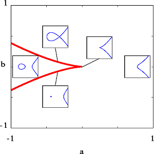
The curve separates the parameter space into two regions. For level curves
indexed by parameters in the region
containing (a,b)=(1,0), the topology of the level set is
that of a line; for level curves indexed by parameters in the
region containing (a,b)=(-1,0) are topologically equivalent to a
circle and a line. For parameter values on the separating curve,
the corresponding level set is singular. This information is summarized in the
image below.

Level sets for Perturbations of the Cusp.
Ending the Session
When you are finished, end this Pisces session by selecting
Quit from the File menu on the Main
Panel.
Next: The Pitchfork Bifurcation
![[Pisces]](../pix/pi.gif) The Pisces Home Page
The Pisces Home Page
Comments to: pisces@geom.umn.edu
Last modified: Sun Nov 26 15:35:10 1995
Copyright © 1995 by
The Geometry Center,
all rights reserved.


![[Pisces]](../pix/pi.gif) The Pisces Home Page
The Pisces Home Page